Summary
In a nutshell
We’ve received criticism from multiple sources that we should model uncertainty more explicitly in our cost-effectiveness analyses. These critics argue that modeling uncertainty, via Monte Carlos or other approaches, would keep us from being fooled by the optimizer’s curse1 and have other benefits.
Our takeaways:
- We think we’re mostly addressing the optimizer’s curse already by skeptically adjusting key model inputs, rather than taking data at face value. However, that’s not always true, and we plan to take steps to ensure we’re doing this more consistently.
- We also plan to make sensitivity checks on our parameters and on bottom-line cost-effectiveness a more routine part of our research. We think this will help surface potential errors in our models and have other transparency and diagnostics benefits.
- Stepping back, we think taking uncertainty more seriously in our work means considering perspectives beyond our model, rather than investing more in modeling. This includes factoring in external sources of evidence and sense checks, expert opinion, historical track records, and qualitative features of organizations.
Ways we could be wrong:
- We don’t know if our parameter adjustments and approach to addressing the optimizer’s curse are correct. Answering this question would require comparing our best guesses to “true” values for parameters, which we typically don’t observe.
- Though we think there are good reasons to consider outside-the-model perspectives, we don’t have a fully formed view of how to bring qualitative arguments to bear across programs in a consistent way. We expect to consider this further as a team.
What is the criticism we’ve received?
In our cost-effectiveness analyses, we typically do not publish uncertainty analyses that show how sensitive our models are to specific parameters or uncertainty ranges on our bottom line cost-effectiveness estimates. We’ve received multiple critiques of this approach:
- Noah Haber argues that, by not modeling uncertainty explicitly, we are subject to the optimizer’s curse. If we take noisy effect sizes, burden, or cost estimates at face value, then the programs that make it over our cost-effectiveness threshold will be those that got lucky draws. In aggregate, this would make us biased toward more uncertain programs. To remedy this, he recommends that (i) we quantify uncertainty in our models by specifying distributions on key parameters and then running Monte Carlo simulations and (ii) we base decisions on a lower bound of the distribution (e.g., the 20th percentile). (more)
- Others2 have argued we’re missing out on other benefits that come from specifying uncertainty. By not specifying uncertainty on key parameters or bottom line cost-effectiveness, we may be missing opportunities to prioritize research on the parameters to which our model is most sensitive and to be fully transparent about how uncertain our estimates are. (more)
What do we think about this criticism?
- We think we’re mostly guarding against the optimizer’s curse by skeptically adjusting key inputs in our models, but we have some room for improvement.
- The optimizer’s curse would be a big problem if we, e.g., took effect sizes from study abstracts or charity costs at face value, plugged them into our models, and then just funded programs that penciled above our cost-effectiveness bar.
- We don’t think we’re doing this. For example, in our vitamin A supplementation cost-effectiveness analysis (CEA), we apply skeptical adjustments to treatment effects to bring them closer to what we consider plausible. In our CEAs more broadly, we triangulate our cost estimates against multiple sources. In general, we try to bring several perspectives to bear on our inputs to ensure they correspond to well-considered posterior beliefs. (more)
- That said, we’ve also identified cases where we’re being insufficiently skeptical of our inputs. For example, in our model, differences in the cost-effectiveness of long-lasting insecticide-treated nets from one country to another are driven substantially by insecticide resistance data. We think it’s likely these data are mostly capturing noise, and so we plan to fix this within the model. (more)
- We prefer the approach of skeptically adjusting inputs over making outside adjustments to the model (as Noah recommends).
- Noah’s recommended approach is to specify distributions on all inputs, then apply an uncertainty-penalizing decision rule (e.g., rank programs based on the 20th percentile of cost-effectiveness). (more)
- Given the way our models are currently set up, we think taking Noah's approach would amount to over-correcting our best guess (i.e., taking it further from what we actually believe), since we think in most cases our inputs reflect our posterior beliefs. (more)
- To avoid this overcorrection, we could strip out our skeptical within-the-model adjustments and then regress our cost-effectiveness estimates toward a program-specific prior. We would prefer this to basing decisions on a fixed percentile, which needn’t correspond to our actual beliefs. In many ways, this would be similar to our current approach. In cases where our evidence is noisier, we think we should adjust to priors or outside considerations. (more)
- However, we prefer our current approach of adjusting specific parameter inputs because we think it’s easier to apply intuition or common sense to individual inputs than bottom-line cost-effectiveness estimates. For example, we think we have better-founded (though still highly subjective) priors for what seems like a plausible effect of deworming on adult income vs. what seems like a reasonable cost-effectiveness estimate for a deworming program. (more)
- We plan to make sensitivity checks on our parameters and on bottom line cost-effectiveness a more routine part of our research.
- We plan to include 25th/75th percentiles on key parameters in our models. We do this on an ad hoc basis now, and we think doing this for each of our models will improve our ability to surface errors, sense-check estimates, and ensure we’re identifying the parameters that are most uncertain. (more)
- In some cases, we’ll also estimate 25th/75th percentiles on cost-effectiveness by running simple Monte Carlo simulations. We think this will drive home how uncertain our bottom-line estimates are (and, in turn, encourage us to view our estimates more skeptically and put weight on other relevant factors). (more)
- Big picture, we think taking uncertainty more seriously in our models means continuing to use “best guess” models and spending more time considering outside-the-model perspectives, rather than trying to beef up our modeling.
- We think the most robust first line of defense against the optimizer’s curse is to ensure the inputs of our models best reflect our well-considered beliefs, as opposed to noisy data that we’ve plugged in uncritically. We think we can make progress on this by (i) improving our guidelines for how to apply skeptical adjustments consistently across programs, (ii) keeping track of assumptions centrally to ensure easy triangulations/across-model gut checks, and (iii) more extensive peer review (both internally and externally) to catch simple mistakes and uncritical judgments. (more)
- While we expect our best-guess cost-effectiveness estimates will continue to be the most important perspective we use to make decisions, we plan to continue evaluating grants from other perspectives (e.g., understanding, intuitively, why some programs are more cost-effective than others, triangulating against expert opinion, and considering the historical track record of interventions and implementers). (more)
How could we be wrong?
- We don’t know if our approach is getting us closer to the truth. For example, we adjust the effect of deworming on adult income downward by approximately 90% to account for our skepticism about the evidence on which we rely. We think this adjustment improves the accuracy of our model, but we don’t know because we don’t observe the “true” effect of deworming on income. For most of the parameters in our model, we won’t know whether we’re getting closer to the truth or not. We may learn more about this through lookbacks and follow-up data. (more)
- We don’t know if Noah’s approach would be better. We think there are practical and conceptual reasons to prefer our approach, but we don’t think we’ll ever know which approach is better, since that would require comparing different models to “true parameters,” which we don’t observe. (more)
- We’re not sure yet what specific “outside-the-model” factors we should rely on and how much weight to put on them. What does model skepticism and putting more weight on non-CEA factors look like? What factors are truly outside of the CEA? We have incorporated non-CEA factors in various grant decisions, but we don't have a fully formed view on how to operationalize this consistently across grants. We expect to consider this further as a team. (more)
- While we think skeptical within-the-model adjustments represent the most sensible way of addressing parameter uncertainty, we recognize that they can’t address structural uncertainty (i.e., whether we’ve chosen the right way to model the program in the first place). But we don’t think the output of a Monte Carlo simulation can address this either, because the resulting distribution only captures uncertainty in modeled parameters. Instead, we view this shortcoming as pointing again to the limitations of relying on a purely quantitative or rules-based approach to decision-making, which gives us more motivation to rely on outside-the-model considerations. (more)
Acknowledgements: We’d like to thank our Change Our Mind contest entrants that focused on our approach to uncertainty: in particular Noah Haber, Alex Bates, Hannah Rokebrand, Sam Nolan, and Tanae Rao. We’d also like to thank Otis Reid, James Snowden, Chris Smith, and Zack Devlin-Foltz for providing feedback on previous versions of this draft.
Published: December 2023
1. GiveWell’s cost-effectiveness models
GiveWell uses cost-effectiveness analysis (CEA) to help rank charities by their impact. At their most basic level, most of our cost-effectiveness models boil down to three key parameters: the burden of a problem (e.g., how many people die from malaria in the Sahel); the cost of an intervention (e.g., the counterfactual cost of distributing an insecticide-treated net); and the effect of the intervention on the problem (e.g., what fraction of malaria deaths are prevented by people sleeping under insecticide-treated nets). These parameters combine multiplicatively to form a cost-effectiveness estimate, which we express as a multiple of direct cash transfers.3
Our cost-effectiveness estimates are the most important (though not only) perspective we use to distinguish between programs (more). We have typically expressed both the inputs and output of our models as point estimates, rather than as probability distributions over a range of values. We’d previously considered quantifying our uncertainty with distributions, but we weren’t convinced that doing so would produce enough decision-relevant information to justify the time and complexity it would add to our work.
2. How and why we plan to quantify uncertainty in our work
2.1 Why we plan to do this
We’ve updated our stance in light of feedback we received from our Change Our Mind contest. We plan to use scenario analysis4 more routinely in our work by specifying 25th and 75th percentiles alongside our central ("best-guess") estimate for key parameters. We already do this to some extent,5 but in a fairly ad hoc way, so we plan to do this more consistently going forward. In some cases (e.g., our top charity CEAs), we also plan to specify basic distributions around these percentiles and run Monte Carlo simulations to produce a distribution of cost-effectiveness estimates.
Since we still plan to rank programs by our best-guess cost-effectiveness estimates (more), we don’t anticipate that this change will lead to large shifts in our grantmaking. However, we think there are other reasons to do this that were well-articulated by our Change Our Mind entrants. In particular, we think quantifying the uncertainty in our inputs and outputs will help with:
- Transparency: We often express our uncertainty qualitatively, saying things like “we feel particularly uncertain about parameter X in our model.” Without putting numbers on this, we recognize that people may interpret this in different ways, which seems bad for transparently conveying our beliefs.
- Prioritization: Running Monte Carlo simulations would allow us to conduct global sensitivity analyses, which would help us to identify the parameters in our models that are most critical in driving variation in our bottom line. This seems good for transparency, but also for informing what we should prioritize in our work. For example, it could help flag areas of our model where additional desk research might be most warranted.
- Sense-checks: We think nudging our researchers to think in terms of distributions would embed healthy sense-checks in our models. For instance, it would help us to interrogate whether our best guess truly represents a mean (vs. a median/mode).6
- Perspective: We don’t think we should be placing all of our weight on our cost-effectiveness estimates when making grant decisions (more), and we think that "seeing" just how uncertain these estimates are will be a helpful reminder to avoid doing this.
2.2 How we plan to do this
We plan to specify 25th and 75th percentiles based on our subjective beliefs, rather than basing them on, e.g., the percentiles implied by the 95% confidence interval reported around a treatment effect. That’s because (i) we don’t have objective measures of uncertainty for most parameters in our model7 and (ii) basing distributions on statistical uncertainty alone seems too restrictive. For example, the 95% confidence interval around a treatment effect can’t account for concerns we have about the identification strategy,8 or whether we understand the underlying drivers of the effect,9 both of which typically influence how confident we feel about the reported effect. So, while the statistical confidence interval might serve as a reasonable first pass estimate, we plan to adjust it in light of these other considerations.
We don’t plan to move our analysis to R, Python, or another programming language. Despite their simplicity, we think spreadsheet-based models have a number of advantages: they allow us to easily "see" the assumptions driving the bottom line (which helps us vet bad assumptions and catch simple mistakes), and they keep our work accessible to people without programming backgrounds, including some of our staff, donors, and subject matter experts. We’re still deciding on the best way to operationalize simple Monte Carlos within this framework,10 but we plan to stick with spreadsheet-based models going forward.
To see what quantifying uncertainty in our models might look like, Figure 1 illustrates a simplified cost-effectiveness model of an Against Malaria Foundation (AMF) long-lasting insecticide-treated net (LLIN) campaign in Uganda, with the 25th and 75th percentiles specified for the key inputs and bottom-line.
| Best-guess | 25th pctile12 | 75th pctile | |
|---|---|---|---|
| Grant size (arbitrary) | $1,000,000 | ||
| Under 5 mortality benefits | |||
| Cost per person under age five reached | $22 | $18 | $3013 |
| Number of people under age five reached | 65,838 | ||
| Years of effective coverage provided by nets | 2.0 | 1.5 | 2.3 |
| Malaria-attributable mortality rate among people under age five | 0.6% | 0.3% | 0.9% |
| Effect of LLIN distributions on deaths related to malaria | 51% | 45% | 58% |
| Percentage of program impact from other benefits | |||
| Mortalities averted for people age five and older | 15% | 10% | 25% |
| Developmental benefits (long-term income increases) | 71% | 37% | 102% |
| Additional adjustments | |||
| Adjustment for additional program benefits and downsides | 38% | 26% | 51% |
| Adjustment for charity-level factors | -4% | -10% | 0% |
| Adjustment for funging | -33% | -58% | -14% |
| Final cost-effectiveness estimates | |||
| Cost-effectiveness (x direct cash transfers) | 18x | 7x | 27x |
3. Why we still plan to use our central (best guess) cost-effectiveness estimates
Noah Haber, one of the winners of our Change Our Mind contest, argues that after running Monte Carlo simulations, we should then base our grantmaking decisions on a lower bound of the resulting distribution (e.g., the 20th percentile). They argue that doing so would help prevent us from over-selecting programs with especially noisy cost-effectiveness estimates (i.e., being susceptible to the "optimizer’s curse").
We don’t think we should do this because we don’t think it would improve our decision-making. To outline our reasoning, we want to explain (i) how we think the optimizer’s curse might crop up in our work, (ii) how the problem is theoretically addressed, (iii) the extent to which our current best-guess estimates already address the problem, and (iv) why we think basing our decisions on a lower bound would risk over-correcting our best-guess (i.e., shifting our decisions further from our actual beliefs), worsening our decision-making.
3.1 The Optimizer’s Curse
We find it easiest to start with the simplest case: imagine that instead of optimizing for cost-effectiveness, GiveWell just funded whichever programs had the largest treatment effects in the global health and development literature. If we took these treatment effects at face value, we think this would be a surefire way we’d be getting "cursed" — we’d be systematically biased toward programs with more uncertain evidence bases.
The theoretical way to address this problem, as outlined in this article, is to not take noisy data at face value, but to instead combine them with a Bayesian prior. This prior should take into account other sources of information beyond the point estimate — be that in the form of other data points or less-structured intuition.
3.2 How we try to address this within the model
3.2.1 Treatment effects
We think our approach to interpreting treatment effects is conceptually similar to this idea. We don’t take literature treatment effects at face value, but instead adjust them based on plausibility caps, other data points, and common-sense intuition. These adjustments enter our models through our internal validity (IV) or replicability adjustments, which make a big difference to our final estimates. For example:
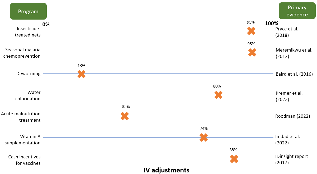
- Deworming: We apply a 13% adjustment (i.e., an 87% downweight) to long-run Miguel and Kremer RCT results which find that childhood deworming increases adult income by 10% per year.14 We’re reluctant to take this estimate at face value because (i) this result has not been replicated elsewhere and (ii) it seems implausibly large given the more muted effects on intermediate outcomes (e.g., years of schooling).15
- Seasonal malaria chemoprevention: We think the evidence base for this program is especially high-quality: the headline treatment effect we use is based on a Cochrane meta-analysis of randomized controlled trials (Meremikwu et al. 2012), all of which seemed well-conducted and reported results in a reasonably consistent direction.16 As such, we take this result more-or-less at face value.
- Vitamin A supplementation: We apply a 74% adjustment to headline results from a Cochrane meta-analysis. We apply a steeper adjustment here in comparison to SMC because we think the underlying trials may be less high-quality,17 and because we have a weaker understanding of the biological mechanisms underlying the mortality effect.18
- Acute malnutrition treatment: The evidence we rely on to estimate the effect of this program is non-randomized (for ethical reasons). We think there are reasons these estimates might be biased upwards,19 so we apply a relatively steep discount to the headline effect.
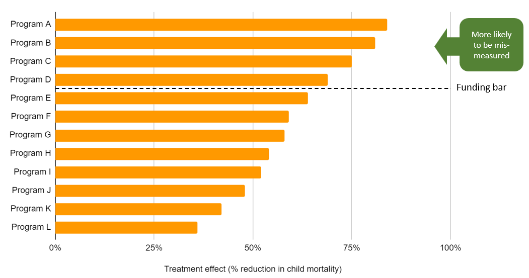
The IV/replicability adjustments we use for the programs to which we direct the most money are illustrated below. These adjustments make a big difference to our final treatment effects — and by extension to our cost-effectiveness estimates — with programs that have (what we consider to be) weaker evidence bases receiving greater penalties. We make these adjustments precisely because of the concern Noah identifies: we don’t want to be biased toward programs whose evidence seems more susceptible to mismeasurement.
In making these adjustments, we don’t use formal Bayesian techniques — i.e., we don’t specify a prior in the form of a mathematical distribution and then update from this in light of the distribution we specify around the treatment effect. We view this as a separate practical question of how best to operationalize a Bayesian approach. We think there are good reasons to prefer a more informal approach: specifying distributions for each parameter would be very time-consuming, would still ultimately be very subjective, and would mean moving our models to a more sophisticated statistical package, which we think would have big consequences for the accessibility of our work. With this being said, we recognize that a more formal approach may force a certain degree of consistency between our models, and so we plan to revisit the relative merits of injecting more formalism into our IV adjustments later this year.
3.2.2 Other parameters
In reality, we don’t just base our decisions on treatment effects; we combine these effects with estimates of program costs, disease burdens, and other factors. The optimizer’s curse would still be a big problem if, to estimate these other parameters, we just plugged noisy data points into our model without subjecting them to scrutiny.
For the most part, we think this is a bad description of how we arrive at our best-guess. For example:
- Costs: We don’t take charity cost information at face value. We typically make adjustments based on expert opinion, additional data points, and triangulations with other programs. For example, to estimate the cost of vitamin A supplementation, we use cross-country averages of cost per supplement administered in cases where we think charity data suggests implausibly low cost estimates;21 to estimate the cost of delivering LLINs, we triangulate AMF's reported costs to procure and distribute LLINs with the Global Fund's cost estimates and a costing study conducted by Malaria Consortium;22 for newer programs, we often benchmark our cost assumptions against our top charity cost estimates (which are generally informed by more data).
- Burden: When we model health-focused programs, we typically estimate burden using third-party estimates produced by the Institute for Health Metrics and Evaluation (IHME). These estimates are quite far-removed from noisy survey data; in most cases, they are the output of Bayesian models (i.e., these are already posterior estimates with Bayesian adjustments baked-in). For example, IHME's malaria incidence estimates come from this paper, which “uses a Bayesian space-time geostatistical model to predict P. falciparum parasite rates [for ages 2-10] for every 5×5 km pixel across all of sub-Saharan Africa annually from 2000–17.”23
- Others: for parameters where we have no primary data to go on whatsoever (e.g., time of policy speed-up for advocacy programs), we typically arrive at our best-guess by (i) starting with a mental model about what timeframe seems reasonable and (ii) incrementally updating away from this model based on conversations with experts, case studies from other countries, etc. Our AMF funging write-up is a good example of this type of approach.24 It explains how we started with a prior expectation of the funding landscape based on global funding gaps, that we incrementally updated from based on conversations with other funders and learning idiosyncratic details about the funding situation of specific countries.
To sum up, we think that for most parameters our best-guess reflects our posterior beliefs — i.e., where we’ve arrived after triangulating between multiple sources of information and gut checking them against our intuition. We think this approach is the most sensible first line of defense in guarding against the optimizer’s curse; it certainly leaves us less susceptible than if we were just putting noisy data points into our models uncritically.
3.3 Why we don’t plan to base decisions on a lower bound
Noah suggests that after running Monte Carlo simulations, we should base decisions on a lower bound of the output (e.g., the 20th percentile; p(> direct cash transfer)). We don’t plan to do this, because we think this would amount to over-updating on our best guess.
To see why, we also find it helpful to go back to the simple case. Imagine that instead of funding the programs that have the largest treatment effects, GiveWell now funds the programs that have the largest ratio of treatment effects to costs.25 Assume also that costs are certain (to get a handle on the intuition). If we’re already skeptically adjusting the treatment effect, we don’t think we should also be skeptically adjusting the cost-effectiveness estimate, since our within-the-model adjustments should already be accounting for noise in the signal. If we base decisions on a lower bound, we think we would over-penalize more uncertain programs like deworming.
To avoid over-correcting, we could:
- Strip out the skeptical adjustments that are already in our models (e.g., IV adjustments; adjustments to charity cost data).
- Input data points at face value (e.g., the 10% deworming treatment effect from Baird et al. 2016; raw cost estimates from the charity).
- Specify distributions around these estimates and run Monte Carlo simulations.
- Do an "all-in" adjustment to this bottom-line. Rather than base decisions on a fixed lower bound (e.g., the 20th percentile), we would prefer to do this more flexibly — i.e., regress our cost-effectiveness estimates toward a program-specific prior, which we think would better incorporate our actual beliefs.26
We think this modeling approach would be possible in principle but a bad idea in practice, because:
- We find it easier to bring intuition/common sense to bear on individual parameters than composite bottom-line cost-effectiveness estimates. For example, we think we have better-founded (though still highly subjective) priors for what seems like a plausible effect of deworming on adult income vs. what seems like a plausible cost-effectiveness estimate for a deworming program.
- If we relied on an all-in adjustment, we don’t think we’d be able to answer basic questions like “what is our best-guess about the effect of deworming on adult income?” That seems bad both for transparency and for enabling basic sense-checks of our beliefs.
- We’re not sure what we would do about parameters that aren’t based on any data. If we think the inputs for these parameters best represent our posterior beliefs, we don’t think we should be indirectly adjusting them based on the distribution that we set around them.
- We think that all-in adjustments would be more liable to basic human error. If we used this approach, our individual parameters would become untethered from intuitive judgment, which we think would make it more likely for bad assumptions and simple mistakes to slip through undetected.
In sum, we think uncertainty in our parameters is best dealt with within the model, rather than via indirect adjustments to the bottom line. We can’t prove this, because we can’t observe the "true" cost-effectiveness of the programs we model, but we feel more confident that our within-the-model adjustments get us closer to the truth because of the difficulties listed above.
4. Pitfalls of this approach (and how we plan to avoid them)
We think there are three main ways our approach could fall short; this section outlines these pitfalls and how we intend to guard against them.
4.1 Inconsistent within-the-model adjustments
The most obvious way we think our approach could fail is if we don’t do the thing we think we ought to be doing — i.e., if we just plug in raw data at face value without subjecting it to common-sense scrutiny. We’ve identified a couple of examples of this kind of mistake in our work, which we think help clarify how the optimizer’s curse might manifest itself — and how we think it’s best dealt with.
Example 1: Insecticide resistance
LLINs are one of the major programs we fund. A key input in our model for this program is the effect of insecticide resistance on LLIN efficacy; put simply, in countries where we think insecticide resistance is more of a concern, we think LLINs are likely to be less cost-effective.
To estimate insecticide resistance across countries, we look at bioassay test results on mosquito mortality. These tests essentially expose mosquitoes to insecticide and record the percentage of mosquitoes that die. The tests are very noisy: in many countries, bioassay test results range from 0% to 100% — i.e., the maximum range possible. To come up with country-specific estimates, we take the average of all tests that have been conducted in each country and do not make any further adjustments to bring the results more in line with our common-sense intuition.
We think we should be wary of estimating insecticide resistance this way. In this case, we think taking noisy data at face value leads to implausibly large cross-country differences. For example, we apply a much larger (59%) adjustment for insecticide resistance in Chad than in Nigeria (14%), despite the fact that the two countries neighbor each other. A more principled way of adjusting for insecticide resistance would be to regress the raw differences in bioassay test result averages toward a common-sense prior, which would capture the intuition that insecticide resistance in Nigeria is probably informative about insecticide resistance in Chad. Other papers effectively take this kind of approach, using Bayesian ensemble models that don’t impose arbitrary cut-offs at country borders.27 When we compare one example of these estimates to ours (Figure 4), we see that the Bayesian model yields much smoother estimates across space — which seems more reasonable.
Panel A: our estimates Panel B: estimates from Moyes et al. (2020)
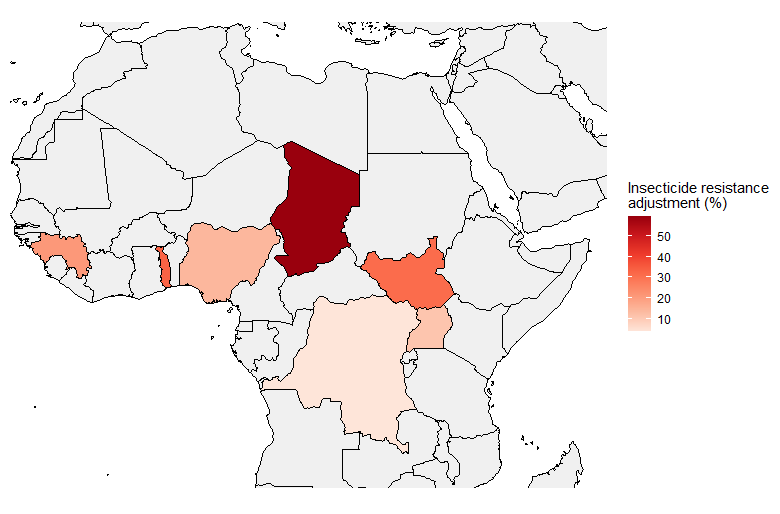

Note on Panel A: larger adjustment = larger reduction in net effectiveness due to insecticide resistance. You can find our underlying calculations here.
Our adjustments for insecticide resistance seem like a clear example where we’re taking noisy data at face value, which leads to an unintuitive bottom-line and potentially misallocated funding decisions. In particular, we may be misallocating funding away from Chad, where our method for aggregating noisy bioassay data may overstate the problem of insecticide resistance. We plan to fix this problem "at the source" — i.e., adjusting our insecticide resistance assumptions until they seem like more defensible best-guesses. This might mean plugging in the third-party modeling estimates directly, or relying on simple heuristics (e.g., regress noisy cross-country data toward a regional mean).
Example 2: Etiology adjustments for the rotavirus vaccine
Another major program area we support is childhood immunization, which we’ve supported via grants to New Incentives and IRD (cash incentives) and Suvita (SMS reminders). To model the cost-effectiveness of these programs, we need to take a stance on the share of deaths that a vaccine prevents for a given disease. This assumption enters our cost-effectiveness estimates through our etiology adjustments; our adjustments for New Incentives can be found here and for Suvita here.
To estimate an etiology adjustment for the rotavirus vaccine, which targets diarrhoeal deaths, we do the following:
- Take raw IHME data on the number of deaths from diarrhea among under 5s in the sub-regions where these programs operate
- Take raw IHME data on the number of deaths from rotavirus (a subset of diarrheal deaths)
- Divide the two to get an estimate of the % of diarrhea deaths in each region that could be targeted by the rotavirus vaccine
As Figure 5 shows, this leads to implausibly large differences between countries; we effectively assume that the rotavirus vaccine is almost completely ineffective at preventing diarrhoeal deaths in India. This seems like a bad assumption; the rotavirus vaccine is part of India’s routine immunization schedule,28 and an RCT in India that administered the rotavirus vaccine to infants showed a 54% reduction in severe gastroenteritis.29
| Bihar (India) | Bauchi (Nigeria) | Bayelsa (Nigeria) | |
|---|---|---|---|
| Number of u5 deaths due to diarrhea | 11,546 | 10,839 | 123 |
| Number of u5 deaths due to rotavirus | 195 | 3,857 | 39 |
| %age of u5 diarrheal deaths caused by pathogens addressed by the rotavirus (etiology adjustment)30 | 2% | 36% | 32% |
In this case, fixing our assumption probably wouldn’t lead to large changes in our cost-effectiveness estimates, as the rotavirus vaccine contributes only a fraction of the benefits across the entire suite of childhood immunizations. However, we think this is a good example of when we should be especially wary of the optimizer’s curse: when we slice and dice data in multiple ways (e.g., by age, region, and disease type), we leave ourselves especially vulnerable to selecting on noise. Again, we think the most sensible place to fix this is within the model, rather than through an indirect adjustment to our bottom line.
4.2 Ignoring counterintuitive differences in our outputs
Suppose we face the following scenario:
- We start out feeling indifferent about program A and program B; both seem equally promising.
- We build a cost-effectiveness model of program A and program B, being careful to interpret raw data skeptically and ensure each input reflects our considered best guess.
- Our model spits out a cost-effectiveness estimate of 20x for program A and 10x for program B.
- This difference feels counterintuitive; we don’t intuitively buy that program A is twice as cost-effective as program B.
Although we think it’d be a mistake to apply a blanket adjustment to this bottom line (e.g., shrink program A to 15x), we also think it’d be a mistake to ignore this intuition entirely. Instead, we think we should use it as a prompt to interrogate our models. Faced with this scenario, we think we should (i) identify the parts of the models that are driving this difference in cost-effectiveness (sensitivity analysis should help with this), and (ii) reconsider whether the differences between these inputs seem intuitively plausible. If not, we should adjust our assumptions until they do.
More broadly, if our cost-effectiveness estimates seem out of step with our intuition, we think this should prompt us to interrogate both our cost-effectiveness estimates and our big-picture intuition. We think we should ideally work from "both directions," until our cost-effectiveness model and our intuition feel more-or-less aligned.
4.3 Placing all of our weight on our cost-effectiveness estimates
Whether we used our approach or Noah’s, we think our cost-effectiveness models would still be subject to two overarching limitations:
- Bad adjustments. Both of our approaches amount to skeptically adjusting evidence we’re more uncertain about. We think we’re more likely to make better adjustments to individual parameters than bottom-line cost-effectiveness estimates (for reasons discussed here), but we’re not going to always get these right. For example, we apply an 87% downweight to the effect of deworming on adult income to get it closer to the "true" effect — but we could be under- or over-correcting.
- Structural uncertainty. Parameter-by-parameter adjustments can’t deal with structural uncertainty (i.e., whether we’ve chosen the right parameters to model in the first place). But we don’t think basing decisions on the 20th percentile of a Monte Carlo simulation can deal with this problem either, since this output is entirely determined by whatever parameters we’ve decided to model in the first place. If we’ve omitted important benefit streams, for instance, both our point estimates and our distributions would be misleading.31
We think these issues point to broader dangers of relying on an entirely quantitative or "rules-based" approach to decision-making and underscore the need to take outside-the-model perspectives seriously. In practice, we do this by asking more qualitative questions alongside our quantitative ones, such as:
- What do experts we trust think about this program? Are they excited by it?
- Do we intuitively buy the theory of change? Can we write down a compelling qualitative case for making this grant?
- Do we trust the management of this charity/implementor to do a good job? Does the grantee have a good track record?
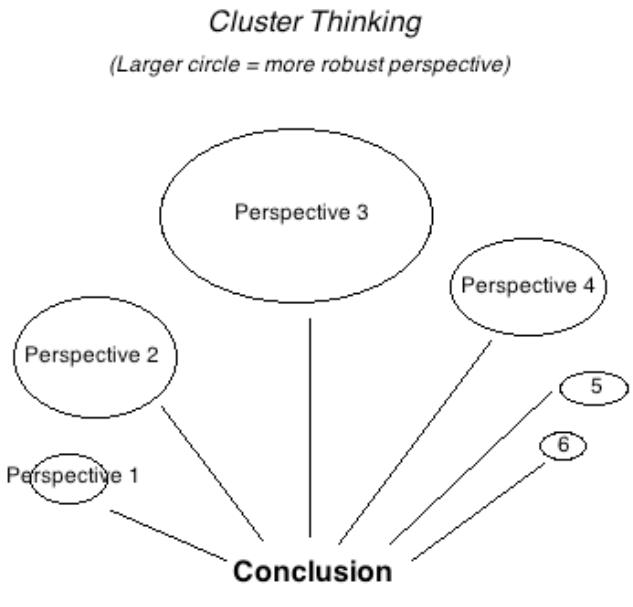
We don’t always try to convert the answers to these questions to the same "currency" as our cost-effectiveness estimates, because we think entertaining multiple perspectives ultimately makes our decision-making more robust. We’ve previously written about this here, and we think these arguments still ring true. In particular, we think cluster-style thinking (Figure 6) handles unknown-unknowns in a more robust way, as we find that expert opinion is often a good predictor of “which way the arguments I haven’t thought of yet will point.” We also think this approach better-reflects successful prediction systems in other contexts, e.g., political forecasting or finance.32 Our view was reaffirmed during this investigation: when we spoke to other decision-makers in finance and philanthropy33 — who we think face similarly high-stakes decisions in uncertain environments — none of them said they would ever base their decisions entirely on the output of a quantitative model. The reasons they gave were similar to the points raised above, e.g., to paraphrase: “we’d be worried about being led astray by a single bad assumption; we know our models are unlikely to be capturing everything we care about.”
We have typically considered our cost-effectiveness estimates to be our most important perspective and expect we will continue to do so. Despite all of the difficulties we have discussed, we still think quantitative models are the most transparent and democratic tool we have to place programs in a comparative framework and make difficult trade-offs between them. But we think there are reasons to be wary about putting all of our eggs in this basket, so we want to leave space for less formal intuition to influence our decision making.
5. How we could be wrong
We think our bottom line on the optimizer’s curse is most likely to be wrong if:
- We’re wrong about our within-the-model adjustments. We adjust raw data points to accord with our intuition and other data sources, but we don’t know whether we’re making the "right" adjustments. For example, we apply an 87% downweight to the effect of deworming on adult income, but we could be under- or over-correcting.
- Basing decisions on a lower bound would get us closer to the truth. Stripping out within-the-model adjustments and basing decisions on a lower bound of a Monte Carlo simulation is another way we could address the optimizer’s curse. We think we have good reasons to prefer our approach (see here), but we can’t prove this definitively.
- Incorporating outside-the-model perspectives introduces inconsistency. Though we think incorporating outside-the-model perspectives seems more conducive to accurate predictions, we recognize that basing decisions entirely on a single model may be more consistent. We think this trade-off is worth it, though we plan to consider ways we can ensure our qualitative lens is being brought to bear consistently across programs.
We think our decision to quantify uncertainty going forward is most likely to be wrong if doing so adds too much time and complexity to our models. We think there are good reasons for doing this (elaborated here), but we’re wary that specifying percentiles and distributions may add clunk to our investigation process, since this may eat into the time we have available for (what we consider to be) the more important tasks of vetting the accuracy of our best guess assumptions, considering outside-the-model perspectives, and exploring new grant opportunities. One alternative to our current proposal would be to just specify 25th and 75th percentiles around key parameters and not run Monte Carlo simulations. We think this would get us a reasonable amount of juice in terms of transparency and sense-checks — and would be faster and simpler. Though we think the additional diagnostics and transparency benefits of doing Monte Carlo simulations seem worth it for our top charities, we may revisit this decision in light of our experiences over the next few months.
6. Next steps
Going forward, we plan to:
- Incorporate sensitivity analysis in published models. We’ve begun this process by incorporating basic sensitivity analysis on key parameters in recent grant and intervention report pages (e.g., zinc/ORS; vitamin A supplementation; MiracleFeet). We’re currently revamping our top charity CEAs to make them more legible, and we plan to incorporate sensitivity analysis and Monte Carlos into these before publishing.
- Keep tabs on assumptions based on raw data. We think taking raw data at face value is a telltale sign that we're being insufficiently skeptical. We’ve identified a few places where we think this is happening here, but we haven’t done a full audit of every assumption in our top charity models (and even less time has been spent looking at our assumptions about programs to which we direct less funding). We’re currently performing a comprehensive internal review of our new top charity CEAs and plan to keep track of any parameters where we think we might be being insufficiently skeptical.
- Revisit IHME burden estimates. While we think these estimates come from models with Bayesian adjustments baked-in, we also don’t think we should be taking these estimates at face value, especially if they diverge from other data sources or our intuition. We’d like to get a better understanding of what’s going on "under the hood" of these estimates, to help us understand whether we should be adjusting them further.
- Improve guidelines for applying skeptical adjustments within our models. A long-term objective of ours is to develop a more uniform approach to how we apply skeptical adjustments in our models. In particular, we think this means (i) revamping our internal guidelines for how to do these adjustments, (ii) keeping track of assumptions centrally to ensure easy triangulations across models, (iii) standardizing our terminology, and (iv) conducting more extensive peer review to ensure we’re being consistent.
Sources
- 1
For an explanation of the optimizer’s curse, refer to the winner of our Change Our Mind contest entry here. A more technical discussion can be found here.
- 2
For example, see this post by Alex Bates on methods for improving uncertainty analysis in cost-effectiveness models, and this post by Hannah Rokebrand et al.
- 3
For example, "10x" means we think a program is 10 times as cost-effective as an equivalent donation to GiveDirectly, an organization that administers unconditional cash transfers to poor households in low-income countries. See here for more information.
- 4
For a further explanation of this concept, refer to Section 2.1 of Alex Bates’ excellent overview of various techniques for quantifying uncertainty in cost-effectiveness analyses.
- 5
We often play with pessimistic and optimistic scenarios internally during our investigation process. In the past, we have occasionally published these alongside our best-guess scenario. For example, in our One Acre Fund BOTEC (stands for "back-of-the-envelope calculation"—what we call our initial, simplified cost-effectiveness models), we calculate cost-effectiveness across a range of more-or-less pessimistic scenarios.
- 6
Since we’re aiming to maximize expected value, all of our inputs should, in theory, correspond to a mean.
- 7
For example, for parameters like “probability another grantmaker funds this program in our absence,” there seems to be nothing equivalent to a statistical confidence interval we could use to parameterize this.
- 8
For example, in general, we feel more skeptical of results that are derived from non-experimental identification strategies vs. randomized controlled trials, since we think the former are more likely to be biased. This skepticism wouldn’t be captured by standard errors or 95% confidence intervals.
- 9
For example, we feel like we have a firmer intuitive grasp of the underlying mechanisms driving the mortality-reducing effects of seasonal malaria chemoprevention compared to the mortality-reducing effects of vitamin A supplementation. We think we should have a more skeptical prior for programs where the causal pathway seems less clear-cut.
- 10
Options we’re considering are: building a custom Google Apps script, using an off-the-shelf Excel plug-in like RiskAMP, or using Dagger, a spreadsheet-based Monte Carlo tool built by Tom Adamczewski.
- 11
This table is partly copied from our most recent cost-effectiveness analysis of AMF's nets program (this model is not yet public). Our finalized estimates may slightly differ from these.
- 12
Note that entries in this column are not meant to be interpreted as "pessimistic" estimates, but rather as the 25th percentile in our probability distribution over an ordered range of possible input values (i.e., numerically lower than our best-guess estimate). Likewise, note that the bottom-line cost-effectiveness estimate in this column is not a function of inputs in this column, but is instead calculated by running Monte Carlo simulations. The same applies to the 75th percentile column.
- 13
For percentiles that aren’t symmetric around our best-guess, we plan to use skewed distributions (e.g., lognormal, two-piece uniform).
- 14
See our calculations for this effect here. For more details on the adjustment we make to deworming RCT results, see our cell note on deworming replicability.
- 15
Baird et al. (2016), Table 2. See our note on our deworming replicability adjustment for how the effects on intermediate outcomes inform our beliefs about the overall effect on income.
- 16
This Cochrane meta-analysis is available here. The RCTs that comprise it pass basic sanity checks, because they include, for example, pre-registration requirements, low attrition rates, transparent randomization procedures, and baseline balance on observables. Likewise, all of the trials that were used to derive the headline treatment effect were listed as having a low risk of bias across the majority of categories (see page 9).
- 17
Many of these trials were conducted in the 1980s and 1990s, before norms like pre-registration were well-established. Our guess is that the quality of randomized controlled trials has generally improved over the years.
- 18
Vitamin A supplementation is hypothesized to reduce mortality primarily by lowering the incidence of measles and diarrhea. When we look at the impact of VAS on these intermediate outcomes, we find smaller effects than the headline effect size would lead us to expect, which makes us more inclined to discount it. See this cell note for more details.
- 19
See the section on unmeasured confounding in our community-based management of acute malnutrition intervention report.
- 20
See our IV adjustments in our CEAs as follows: LLINs, SMC, Deworming, Chlorination, VAS. Our malnutrition adjustment is part of our latest CEA for acute malnutrition treatment, which is not yet public. Our IV adjustment for cash incentives for vaccines is still a work-in-progress: we plan to update our model as soon as our bottom-line is finalized.
- 21
See, for example, our cost estimates for the Democratic Republic of the Congo, Kenya, and Nigeria here.
- 22
Our calculations for estimating AMF's LLIN costs are non-public, because they rely on Global Fund data that we do not have permission to publish.
- 23
While we think Bayesian adjustments are already baked into IHME estimates, there is a separate question about whether these are the "right" adjustments. See here for how we plan to dig into this.
- 24
For an explanation of funging, see here.
- 25
This might be considered a very rough proxy of cost-effectiveness.
- 26
Whether we did this formally or informally, we think a Bayesian-style approach would be a more principled way of implementing an all-in adjustment compared to basing decisions on an arbitrary percentile. Put another way, if our central cost-effectiveness estimates don’t correspond to our intuition (because we’re not skeptically adjusting the inputs), we should adjust them until they do, rather than make a fixed adjustment which needn’t correspond to our actual beliefs. This approach better reflects how we treat, for example, uncertain treatment effects.
- 27
See, for example, Moyes et al. (2020).
- 28
India routine immunization schedule, UNICEF.
- 29
“71 events of severe rotavirus gastroenteritis were reported in 4752 person-years in infants in the vaccine group compared with 76 events in 2360 person-years in those in the placebo group; vaccine efficacy against severe rotavirus gastroenteritis was 53·6% (95% CI 35·0-66·9; p=0·0013)”, Bhandari et al. (2014), p. 1.
- 30
Note that the etiology adjustments in this row may not exactly match the adjustments in our actual models because those models also incorporate additional adjustments. We've simplified these calculations for ease of exposition.
- 31
In general, penalizing uncertainty via the 20th percentile cost-effectiveness estimate could be misleading if the fraction of quantified uncertainty differed between programs. We could keep throwing in parameters—trying to capture more and more of the "true" model—but we’d have to draw a line somewhere. In practice, we try to be consistent by considering the same type of benefits across programs (e.g., mortality, morbidity and income effects), and being consistent about where we cut off benefits in space and time (e.g., assuming a 40-year time horizon for income effects). We think these are sensible rules-of-thumb, but we shouldn’t assume that we’ll always be capturing a consistent fraction of consequences across programs.
- 32
E.g., Political forecaster Nate Silver writes: “Even though foxes, myself included, aren’t really a conformist lot, we get worried anytime our forecasts differ radically from those being produced by our competitors… Quite a lot of evidence suggests that aggregate or group forecasts are more accurate than individual ones.” Nate Silver, The Signal and the Noise, p. 66.
Placing 100% weight on our cost-effectiveness model feels akin to placing 100% weight on a single forecast (and not taking into account other people’s predictions or revealed preferences).
- 33
We spoke to decision-makers at Commonweal Ventures (social impact VC), Asterion Industrial Partners (private equity), Lazard (asset management), and PATH (global health philanthropy).